Topologies
Sabaody implements all the topologies provided by PyGMO version 1.
One-way Ring
This topology is a directed cycle - migrants only flow in one direction around the ring.
In [1]:
#import tellurium
#from sabaody import TopologyFactory
from sabaody.topology import TopologyFactory

# dummy problem and algorithm for generated islands
class NoProblem:
    pass
class NoAlgo:
    pass

# create one way ring topology
f = TopologyFactory(NoProblem)
one_way_ring = f.createOneWayRing(NoAlgo,6)

# draw the topology
import networkx as nx
nx.draw(one_way_ring, pos=nx.spring_layout(one_way_ring,0.01,random_state=0))
import matplotlib
matplotlib.pyplot.show()
<Figure size 640x480 with 1 Axes>
Bidirectional ring
Like the one-way ring but migrants can flow in either direction.
In [2]:
bidir_ring = f.createBidirRing(NoAlgo,6)
nx.draw(bidir_ring, pos=nx.spring_layout(bidir_ring,0.01,random_state=0))
matplotlib.pyplot.show()
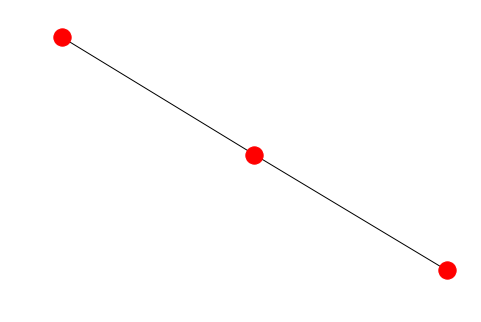
Bidirectional chain
A simple linear topology.
In [3]:
bidir_chain = f.createBidirChain(NoAlgo,3)
nx.draw(bidir_chain, pos=nx.spring_layout(bidir_chain,0.01,random_state=0))
matplotlib.pyplot.show()
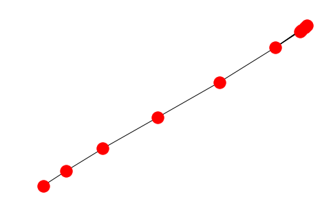
Lollipop
A lollipop is a complete graph connected to a linear chain.
In [4]:
lollipop = f.createLollipop(NoAlgo,complete_subgraph_size=5,chain_size=5)
nx.draw(lollipop, pos=nx.spring_layout(lollipop,0.01,random_state=0))
matplotlib.pyplot.show()
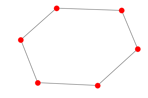
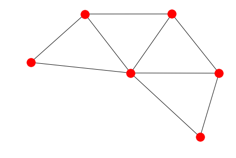
Rim
A bidirectional cycle with all nodes connected to a single node on the rim.
In [5]:
rim = f.createRim(NoAlgo,6)
nx.draw(rim, pos=nx.spring_layout(rim,0.05,random_state=0))
matplotlib.pyplot.show()
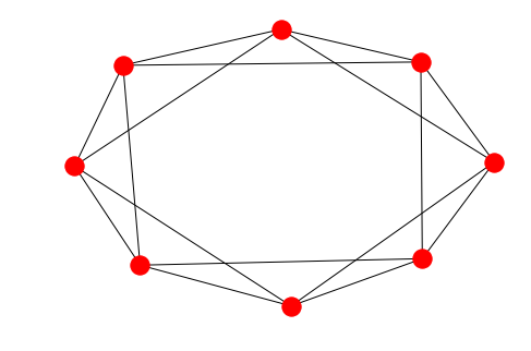
1-2 Ring
A bidirectional cycle where each node is also connected to its next-nearest neighbor.
In [6]:
ring12 = f.create_12_Ring(NoAlgo,8)
nx.draw(ring12, pos=nx.spring_layout(ring12,0.1,random_state=0))
matplotlib.pyplot.show()
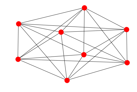
1-2-3 Ring
A topology where each node is connect to its next-nearest neighbor, as in a 1-2 ring, but is also additionally connected to its respective third neighbors.
In [7]:
ring123 = f.create_123_Ring(NoAlgo,8)
nx.draw(ring123, pos=nx.spring_layout(ring123,0.1,random_state=0))
matplotlib.pyplot.show()
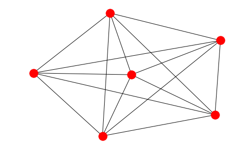
Fully Connected (Complete Graph)
A topology where each node is connected to every other node (i.e. a complete graph).
In [8]:
fully_connected = f.createFullyConnected(NoAlgo,6)
nx.draw(fully_connected, pos=nx.spring_layout(fully_connected,0.1,random_state=0))
matplotlib.pyplot.show()
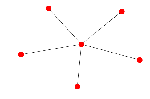
Broadcast
A collection of nodes not connected to each other but to a central node.
In [9]:
broadcast = f.createBroadcast(NoAlgo,6)
nx.draw(broadcast, pos=nx.spring_layout(broadcast,0.1,random_state=0))
matplotlib.pyplot.show()
Hypercube
A topology defined by the hypercube of dimension \(N\), with \(2^N\) verticies and \(N\cdot2^{N-1}\) edges.
In [10]:
hypercube = f.createHypercube(NoAlgo,4)
nx.draw(hypercube, pos=nx.spring_layout(hypercube,0.1,random_state=0))
matplotlib.pyplot.show()
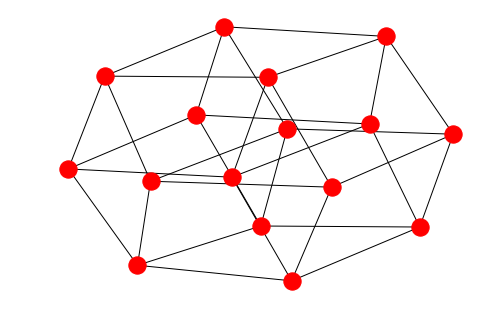
Watts-Strogats
A Watts-strogats graph tends to exhibit small-world effects.
In [11]:
watts_strogatz = f.createWattsStrogatz(NoAlgo,num_nodes=16,k=8,p=0.1,seed=1)
nx.draw(watts_strogatz, pos=nx.spring_layout(watts_strogatz,0.1,random_state=0))
matplotlib.pyplot.show()
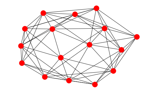
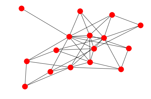
Erdős-Rényi
The oft-cited original random graph algorithm, the Erdős-Rényi method samples graphs uniformly from a distribution of \(N\) nodes and \(M\) edges. That is, all graphs with \(N\) nodes and \(M\) edges are equally likely.
In [12]:
erdos_renyi = f.createErdosRenyi(NoAlgo,num_nodes=16,p=0.5,seed=1)
nx.draw(erdos_renyi, pos=nx.spring_layout(erdos_renyi,0.1,random_state=0))
matplotlib.pyplot.show()
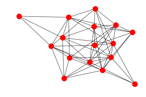
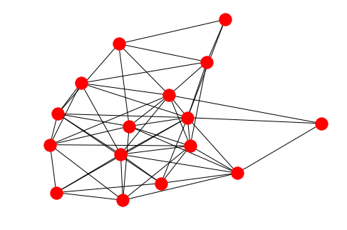
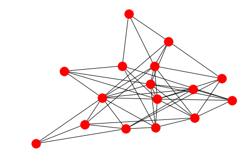
Barabási-Albert
Designed to exhibit the same power-law scaling behavior found in many naturally occurring networks (such as genetic circuits, social networks, and the World Wide Web), the Barabási-Albert method constructs graphs by adding new edges to nodes based on the number of edges already connected to the node. The end result is a graph with a small number of centralized “hubs” harboring the majority of connections.
References:
Barabási, A. L., & Albert, R. (1999). Emergence of scaling in random networks. Science, 286(5439), 509-512.
In [13]:
barabasi_albert = f.createBarabasiAlbert(NoAlgo,num_nodes=16,m=3,seed=1)
nx.draw(barabasi_albert, pos=nx.spring_layout(barabasi_albert,0.1,random_state=0))
matplotlib.pyplot.show()
Extended Barabási-Albert
The original Barabási-Albert algorithm spawned many variants. In this
popular variant, implemented as extended_barabasi_albert_graph in
networkx, the graph is grown via three processes, which can be selected
probabilistically at each step of the algorithm:
- Addition of m new edges with probability p
- Rewiring of m edges with probability q
- Addition of a new node with probability 1 - p - q
Of course, the processes are mutually exclusive and \(p + q < 1\). This method can operate in a scale-free regime (\(q = 0\)) or an exponential regime (\(q \rightarrow 1\)).
References:
Albert, R., & Barabási, A. L. (2000). Topology of Evolving Networks: Local Events and Universality. Physical Review Letters 85(24), 5234.
In [14]:
extended_barabasi_albert = f.createExtendedBarabasiAlbert(NoAlgo,16,m=3,p=0.3,q=0.1,seed=1)
nx.draw(extended_barabasi_albert, pos=nx.spring_layout(extended_barabasi_albert,0.1,random_state=0))
matplotlib.pyplot.show()
Extended Ageing Barabási-Albert
Identical to the extended Barabási-Albert but nodes older than
max_age cannot be connected to, effectively capping the connectivity
of individual nodes. This topology is intended to fill the role of the
ageing clustered Barabási-Albert topology from
PyGMO.
However, the PyGMO version uses an unknown variant of the
Barabási-Albert for their “clustered” Barabási-Albert model and this
one. For our implementation, we use the well-known “local events” model
referenced above (Phys Rev. Letters, Dec. 2000).
In [15]:
ageing_barabasi_albert = f.createAgeingExtendedBarabasiAlbert(NoAlgo,n=16,m=3,p=0.3,q=0.1,max_age=10,seed=1)
nx.draw(ageing_barabasi_albert, pos=nx.spring_layout(ageing_barabasi_albert,0.1,random_state=0))
matplotlib.pyplot.show()